Nine LLM Inference Metrics That Reveal Latency, Throughput, and Service Quality
- Cargo
- Machine Learning
- Shipped
- Shipper
- Bala Priya C
- Readers
- 609
Separate first-token delay, streaming speed, system throughput, and SLO success to see where inference performance helps or hurts users.
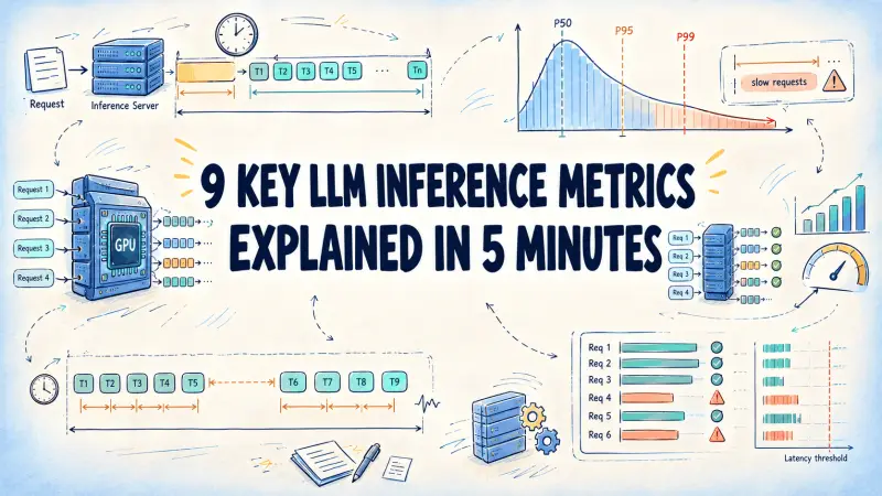
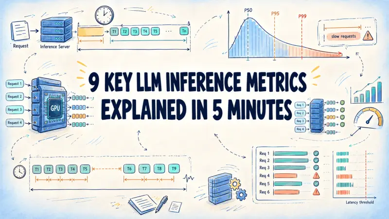
A high token rate can hide a sluggish user experience. An inference server may produce many tokens overall while making each user wait too long for the first one, or while streaming unevenly under concurrent load. Evaluating serving performance therefore takes more than a single throughput figure: it means measuring the start of a response, the pace of generation, variation across requests, and the share that meet service targets.
Nine metrics provide that view. The first five describe one request; percentiles summarize latency across requests; requests per second and tokens per second measure server output; and goodput counts requests that satisfy latency objectives.
Start with the request timeline
Four values anchor the latency calculations: \(t_{\text{send}}\), when the client sends a request; \(t_{\text{first}}\), when its first output token arrives; \(t_{\text{last}}\), when its last token arrives; and \(N_{\text{out}}\), the number of output tokens. For inter-token latency, record the arrival time \(t_j\) of each token, with \(t_1=t_{\text{first}}\) and \(t_{N_{\text{out}}}=t_{\text{last}}\).
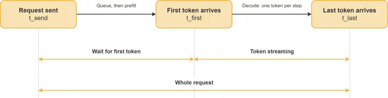
Before the first token arrives, time may be spent in a server queue and in prefill, where the model processes the prompt. Afterward, decoding produces the output step by step, typically one token per step. The distinction matters operationally: a long initial wait points to a different part of the serving path than a slow or interrupted stream.
Latency: response start, stream, and total wait
Time to first token (TTFT) measures the delay from sending a request until its first output token arrives:
\[\text{TTFT}=t_{\text{first}}-t_{\text{send}}\]
TTFT includes network travel, queueing, and prompt processing. It can rise with server load and prompt length. For interactive chat, it directly captures how long a user waits before seeing any response.
End-to-end latency (E2E) runs from request submission to the final output token:
\[\text{E2E}=t_{\text{last}}-t_{\text{send}}\]
This is the full response wait. It combines TTFT with the time spent streaming the remaining output.
Token generation time isolates that streaming portion:
\[\text{TokenGen}=t_{\text{last}}-t_{\text{first}}=\text{E2E}-\text{TTFT}\]
Longer answers naturally take more time to generate, so this value alone doesn't describe the stream's pace. For that, use time per output token.
Time per output token (TPOT) averages the gaps after the first token:
\[\text{TPOT}=\frac{\text{E2E}-\text{TTFT}}{N_{\text{out}}-1}=\frac{\text{TokenGen}}{N_{\text{out}}-1}\]
The denominator excludes the first token because its wait is already captured by TTFT. TPOT is undefined for a one-token response. Definitions can differ across benchmarking tools: some include TTFT in the average, while others use inter-token latency as another name for TPOT. Check the precise definition before comparing measurements. The Databricks inference performance guidance discusses TPOT in the context of serving performance.
Inter-token latency (ITL) records each individual gap between consecutive tokens:
\[\text{ITL}_j=t_{j+1}-t_j,\quad j=1,\dots,N_{\text{out}}-1\]
For a single request, the mean of its ITL values equals its TPOT. Across \(R\) requests, however, the averages give different weight to the data. If request \(i\) produces \(N_i\) tokens, mean ITL counts every gap, while mean TPOT gives each request one vote:
\[\overline{\text{ITL}}=\frac{\sum_{i=1}^{R}\sum_{j=1}^{N_i-1}\text{ITL}_{i,j}}{\sum_{i=1}^{R}(N_i-1)}\qquad\overline{\text{TPOT}}=\frac{1}{R}\sum_{i=1}^{R}\text{TPOT}_i\]
As a result, long responses have more influence on mean ITL, while short and long responses count equally in mean TPOT. Keeping individual ITL samples also makes pauses within a response visible, which an average can conceal.
Summarize latency across requests
Each latency metric varies from request to request, so report a distribution rather than relying on one sample. The mean gives the arithmetic average and is affected by outliers. The median, or P50, marks the point at or below which half of requests fall. P99 marks the point at or below which 99% fall, exposing slow tail behavior; P90 and P95 offer less extreme views.
Calculate these statistics separately for TTFT, TPOT, and E2E. With \(N\) measurements sorted in ascending order, the nearest-rank percentile is:
\[\bar{x}=\frac{1}{N}\sum_{i=1}^{N}x_i\qquad P_k=x_{\left(\left\lceil\frac{k}{100}N\right\rceil\right)}\]
For a multi-server deployment, calculate percentiles from the combined raw samples. Averaging per-server P99 values does not produce the P99 of traffic across the whole deployment.
Measure capacity and service quality
Throughput metrics use a measurement window from \(t_{\text{start}}\) to \(t_{\text{end}}\). Requests per second (RPS) counts completed requests per unit of wall-clock time:
\[\text{RPS}=\frac{N_{\text{completed}}}{t_{\text{end}}-t_{\text{start}}}\]
RPS doesn't account for how much work each request contains. Compare it across runs only when prompt and output lengths have a similar mix.
Tokens per second (TPS) reports token processing rates, with separate forms for input and output. If \(N_{\text{prompt},i}\) is the number of prompt tokens in request \(i\), then:
\[\text{TPS}_{\text{out}}=\frac{\sum_i N_{\text{out},i}}{t_{\text{end}}-t_{\text{start}}}\qquad\text{TPS}_{\text{in}}=\frac{\sum_i N_{\text{prompt},i}}{t_{\text{end}}-t_{\text{start}}}\]
Always specify which rate a TPS figure represents. Long prompts and short replies can yield high input TPS without much output generation.
Goodput counts completed requests that meet every defined service-level objective (SLO), such as limits on TTFT, TPOT, or E2E. In the vLLM serving benchmark, it is a rate of successful requests. The DistServe paper uses the term for a different quantity: the maximum request rate a GPU can sustain within latency constraints.
For limits \(s_{\text{ttft}}\), \(s_{\text{tpot}}\), and \(s_{\text{e2e}}\), request \(i\) qualifies when it satisfies all three:
\[\text{TTFT}_i\le s_{\text{ttft}}\land\text{TPOT}_i\le s_{\text{tpot}}\land\text{E2E}_i\le s_{\text{e2e}}\]
If \(N_{\text{good}}\) requests qualify during the measurement window, goodput is:
\[\text{Goodput}=\frac{N_{\text{good}}}{t_{\text{end}}-t_{\text{start}}}\]
Goodput cannot exceed RPS. Their difference is the rate of completed requests that miss at least one target. Taken together, the metrics separate response startup, stream behavior, total latency, workload volume, and SLO success. That separation makes performance results easier to interpret—and helps identify which part of the serving experience needs attention.